Say a trader tells you the strategy got better last month. Ask what it looked like before and you get a shrug, a memory of a rough patch, and a screenshot of the best week. There's no before photo, so nothing can be compared and nothing can be disproved.
A baseline is that before photo, with a timestamp. More precisely, it's a documented reference period that records the outcomes and the conditions that generated them: net return after costs, dispersion, drawdown, and the market state each trade happened in. Get the definitions right once and later comparisons become almost mechanical.
| Metric |
What to record |
Why it belongs in the baseline |
| Net return |
Return after fees, slippage and funding for the full period |
Shows what you kept, not what the chart showed |
| Return dispersion |
Standard deviation of per-trade or per-day returns |
Separates normal swings from real change |
| Maximum drawdown |
Largest peak-to-trough fall in the equity curve |
Shows the loss you actually had to absorb |
| Win rate and average R-multiple |
Share of winning trades and average result per unit of risk |
Pairs frequency with size, because win rate alone can mislead |
| Expectancy |
Average net R per trade, weighting wins and losses |
Tells you whether the edge is positive |
| Profit factor |
Gross profit divided by gross loss |
Quick check of how wins and losses balance |
| Average holding time |
Mean time in position per trade |
Reveals drift toward longer or shorter trades |
| Fees and slippage |
Total cost per trade and as a share of gross return |
Keeps execution costs inside the baseline |
Win rate is the metric that misleads most. A 70 percent win rate with tiny winners and a few large losers can lose money steadily, while a 35 percent win rate with a 3R average winner can compound. Recording the win rate next to the average R-multiple forces the two facts to sit together. A success rate with no reference distribution behind it tells you very little, which is why even the definition of a healthy win rate for Solana wallets shifts with what counts as a win and how large each one is.
Net return after fees, slippage and funding is the figure that decides whether any of the rest matters. Gross return flatters a high-frequency style that pays its edge back in costs. Our breakdown of trading metrics beyond win rate covers the measures that fill out the rest of the set.
The comparability rule: every period in the baseline uses the same definitions, the same cost treatment and the same calculation method. Change any of the three and you have a new baseline, not an updated one.
The build is less work than traders expect, and almost all of the value sits in the order of the steps. Statistical process-control practice is explicit about that order: gather and graph baseline data for every chosen measure before improvement work begins, and confirm the measure is stable before its average is trusted as a reference point. A later result that lands outside the established control limits is stronger evidence of a real shift than a simple comparison with one prior observation, as this SAS statistical process-control paper lays out.
Here's the whole sequence in one view.
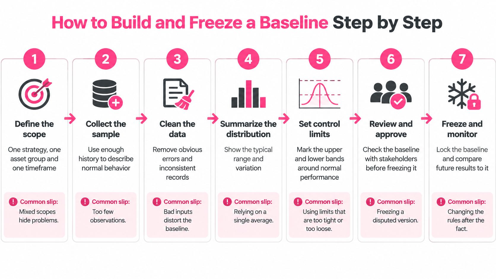
1. Define the scope narrowly. One strategy, one asset group, one timeframe. A baseline that mixes a scalping book and a swing book produces an average that describes neither. The usual slip is mixing spot and perpetual positions in an untagged pile, so borrowing and funding contaminate the result.
2. Export every closed trade in the period. Include the setups you skipped if you logged them, because the trades you didn't take are part of the process. The familiar slip is keeping only the winners, which turns a baseline into a highlight reel.
3. Tag each trade by regime, asset, setup and emotion before you calculate anything. Tagging afterwards lets you sort the data to fit a story you've already decided on. Market regime at entry, venue, and psychological state all belong in the row.
4. Check whether the series is stable. Plot per-trade R or rolling expectancy and look at the shape. A series that drifts upward across the window, or swings between extremes, hasn't settled, and averaging it manufactures a reference point that never existed. Slip: averaging an unstable stretch and calling it normal.
5. Calculate the core metrics on the stable window only, with one fixed method. Net return, dispersion, maximum drawdown, win rate, average R-multiple, expectancy, profit factor, holding time, and total costs. One calculation method, applied identically every time you rebuild.
6. Freeze the document. Give it start and end dates, the calculated values, and the center line with upper and lower control limits, typically the mean plus or minus three standard deviations of the series. Then state plainly that no improvement changes take effect until this version is dated and saved.
7. Lock the method itself. Any later change to definitions, cost treatment or trade inclusion creates a new baseline rather than an edit to the old one. This is the step that protects you from your future self, who will be tempted to tidy history after a bad quarter.
A frozen entry reads like this:
Baseline v1, frozen 1 April 2026: Jan to Mar 2026, 84 trades, expectancy +0.31R, maximum drawdown 9.4 percent, profit factor 1.42, average hold 6.3 hours, net return after fees and funding +4.8 percent.
After that, you repeat the same review on the same window length each month: last three months measured against the frozen distribution. A spreadsheet handles this comfortably. Whatever holds your journal should export every trade to CSV or JSON so the baseline stays portable and yours; the journal in our Pro plan supports CSV import, read-only account sync, psychology tags per trade, and a dashboard with equity curves and R-multiples.
Twelve trades look like a track record and behave like a coin flip. With a small sample you can't see how much your results normally vary, which means you can't tell a genuine improvement from an ordinary hot streak. A baseline needs enough observations across normal conditions to expose the spread, the trend and the outliers.
Measurement practice gives a useful anchor. NIST's measurement-quality handbook notes that establishing an accepted value for a control-chart baseline required at least 100 check-standard values in its example. That example comes from calibrating instruments, not from trading, so treat the figure as a conservative target rather than a rule. Around 100 closed trades is a sensible aim where your history allows it.
| Closed trades in window |
Baseline status |
Action |
| Fewer than 30 |
Provisional |
Keep logging, change no rules, widen expectations |
| 100 or more |
Full baseline |
Freeze center line and control limits |
| Break of three months or platform change |
New sample |
Start a new window |
Between 30 and 100, you have something usable for gross observations but not for fine distinctions. Use that window to describe the shape of your results, not to rank setups.
Run the split-test before you freeze. Break the window into its first and last third and chart both. If the later third sits consistently above or below the earlier one, the process is already shifting and the honest move is to split the window rather than average two different behaviours together. A trend inside your baseline means your baseline is describing a moving target.
Breaks matter too. A three month pause, a platform migration, or a change in fee tier starts a new sample, because the conditions that produced the old numbers are gone. If the sample is too small to support a decision, the decision is to keep logging without touching your rules. That's an answer, not a delay. The mechanics of getting to a usable sample size are covered in our guide to sample size in crypto trading.
A trader shows a journal with a 58 percent win rate across the whole account and concludes the process is sound. Split the same journal and the picture breaks apart: 31 percent on low-liquidity altcoins during thin weekend sessions, well above average on two majors during trending weeks. The aggregate rate was hiding the segment that was bleeding.
That's the argument for building separate baselines by regime (trending, ranging, high volatility), by asset group, by timeframe and by setup. Set a minimum trade count per bucket, something like 20, so no conclusion rests on three trades. Where a bucket is too thin, keep it provisional and say so.
Record the conditions, not just the outcome. In the first half of 2026, average daily derivatives volume fell 15.7 percent year over year to $193.8 billion and average open interest declined 10.0 percent to $112.7 billion, according to the 2026 half-year derivatives market report. A baseline built in a busier market describes a market that no longer exists. Volatility, liquidity, funding, open interest, exposure and regime belong in the row next to the trade.
Separate skill from carry and friction. Positive funding pays shorts and charges longs, so a short-heavy book can look sharper than it is while funding runs one way and look mediocre when it flips. Fees and slippage stack on top and can reverse a strategy that appears profitable at gross. A trader who takes fewer trades and avoids degraded liquidity or crowded positioning may be improving even while returns fall.
Which brings the baseline to the question it exists to answer.
Did the trader improve, or did the market simply become easier to trade?
If your baseline can't distinguish those two, it's a mood ring with a decimal point.
Raw return ranks strategies poorly. A strategy returning 20 percent with 30 percent volatility can be inferior to one returning 12 percent with 10 percent volatility, depending on the risk-free rate and the observation frequency. Ranking by the headline number rewards borrowed exposure and market direction, not decisions.
The Sharpe ratio fixes part of that by dividing excess return over the risk-free rate by return volatility. The information ratio applies the same logic relative to a chosen benchmark, dividing mean excess return over that benchmark by the variability of the excess. CFA Institute guidance on the Sharpe ratio and the information ratio sets out both definitions and the frequency problem that comes with them, since annualizing daily Sharpe ratios is where a lot of comparisons go wrong.
A benchmark has to pass a test before it means anything. CFA guidance holds that a valid benchmark should be unambiguous, investable, measurable, appropriate, specified in advance and accountable. For crypto derivatives, that means documenting whether you compare against a spot index, a perpetual-futures return, cash plus the risk-free rate, or a strategy-specific neutral benchmark, and matching it to the assets, position size and holding period you use in practice.
| Benchmark |
Best used when |
Main caveat to document |
| Spot index of the traded assets |
You trade the underlying assets without leverage |
Does not capture funding or leverage effects |
| Perpetual-futures return |
Your strategy is directional and leveraged on the same contracts |
Includes funding, so fees and funding must match across periods |
| Cash plus risk-free rate |
You want to test whether trading beats holding cash |
Ignores market direction, so beta exposure can look like skill |
| Strategy-specific neutral benchmark |
Your strategy aims for market-neutral results |
Must be defined before the baseline is frozen |
| Buy and hold of the same asset |
You want to know if active trading added value |
Penalises short or hedged strategies designed to lose in rallies |
Two more figures earn a place beside the core set. Beta measures your sensitivity to benchmark moves, and Jensen's alpha estimates return beyond the theoretical compensation for systematic risk. A positive return with a beta of 1.3 during a strong market is mostly exposure.
The consistency rule: report absolute return, benchmark-relative return, Sharpe, maximum drawdown, downside volatility, exposure, beta and alpha together, with identical fee and funding treatment in every period. Without that, an improvement may just be more leverage in a friendlier funding regime.
Our performance analytics apply the same discipline, and the risk-adjusted returns in crypto piece walks through how to read those figures without fooling yourself.
The instinct after a rule change is to compare the next result with the last one that hurt. One profitable trade proves nothing about a process, and one bad week disproves nothing either. Post-change results have to be read against the pre-change distribution, not against a single observation in either direction.
Control limits earn their keep here. If the measure stays inside the bands you froze, the result is ordinary variation and the correct response is to keep collecting data. Repeated observations outside those limits, especially on the same side, are grounds for investigation: something about the process has changed. The comparison also has to match on regime, because a strong month in a trending market measured against a baseline built mostly in ranging conditions can look like skill when it is mostly weather.
Thrive's journal and performance dashboard keep closed trades, equity curves and R-multiples in one place, so a breached limit leads straight back to the trades that caused it.
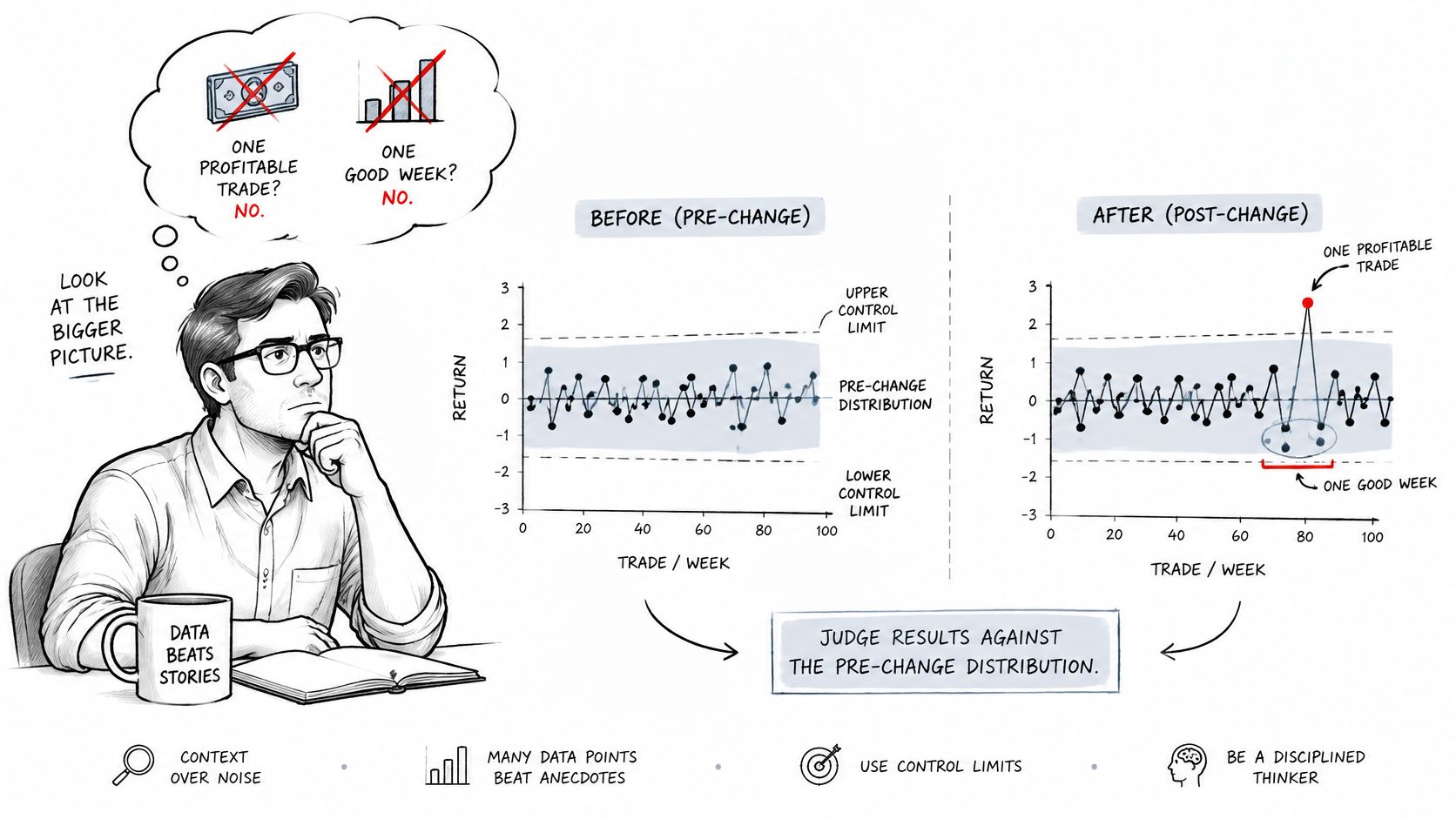
Attribution is the second half of the problem. Change your entry rules and the asset mix shifts in the same month, and you cannot tell which of the two moved your numbers. The same applies to state of mind: a rule change and a rough personal patch in the same stretch will blend together unless emotions were tagged per trade. Log changes at the time of the trade so the comparison stays possible later.
Consistent reporting is what makes a history usable. Before the late 1980s there were no broadly accepted standards for calculating and presenting investment results. Concern about misuse of performance information led the U.S. Securities and Exchange Commission to consider regulatory action in 1987, and the industry standardised instead, with the first Global Investment Performance Standards published in April 1999. Those standards require an investment firm to present at least five years of annual, standards-compliant performance, or since inception if younger, as the 2020 GIPS standards for asset owners set out. The lesson transfers directly: disclose the period, fees, cash flows and benchmark, and calculate it the same way every time.
Five misreadings account for most of the damage:
- Editing the baseline after a bad month. The reference point moves and every later comparison flatters you.
- Comparing a two-week window against a one-year baseline. Different lengths capture different amounts of luck.
- Reading a trending month against a ranging baseline. A friendlier market can masquerade as a better process, so compare each period with the slice of the baseline built under similar conditions.
- Moving the start date to make the numbers look better. If the window needs adjusting, the honest move is a new baseline with a dated reason, not a quiet rewrite.
- Declaring victory from one profitable week. One observation is a data point, not a distribution.
Match each review window to the baseline slice that fits it, and read every post-change result against the frozen figures without editing them. When a genuine method change is warranted, freeze a new baseline, date it, and keep the old one in the file so the chain of comparisons survives.
Baselines only work when the data behind them is complete, and our journal is built for exactly that: CSV import, read-only exchange sync, psychology tags on every trade, and a performance dashboard that sets the equity curve next to the market conditions each trade was taken in. Export the same trade data you reviewed, save a first baseline from it, and compare each month's results against your own saved figures. Visit Thrive to start yours.