Say you run a small shop. Saturday carries the week and Tuesday loses money, yet the weekly total still prints a profit. Your trade log works the same way. A green month can be one busy overlap and several quiet sessions that never paid for the risk. Splitting closed trades into periods shows when the edge shows up and when it fades.
The window is the choice that changes the picture. A single session pins the clock, but each slice holds few trades, so one winner can swing the whole bucket. A full quarter gives steadier counts and blurs the hour the edge appeared. Crypto trades around the clock, so session labels are conventions, not exchange closes. Daylight saving also nudges local clocks against UTC, which is why the windows below stay in UTC and stay approximate.
Start with two or three periods. Testing every slice at once almost guarantees that one of them looks special.
| Period |
Window to use |
Minimum closed trades per bucket |
What it can reveal |
| Asia session |
00:00-08:00 UTC |
20 |
Whether results depend on the quieter Asian hours |
| London session |
07:00-16:00 UTC |
20 |
Whether results depend on European trading |
| New York session |
12:00-21:00 UTC |
20 |
Whether results depend on US trading |
| London and New York overlap |
12:00-16:00 UTC |
20 |
Results during the busiest hours of the day |
| Day of week |
Monday to Sunday |
20 |
Recurring weekday patterns |
| Weekday versus weekend |
Monday-Friday against Saturday-Sunday |
40 |
Whether thinner weekend liquidity changes your results |
| Week of month |
Days 1-7, 8-14, 15-21 and 22 to month end |
20 |
Whether results cluster around a point in the monthly cycle |
Twenty closed trades is the floor for a session, a weekday, or a week-of-month slice. Forty is the floor when you compare weekdays with the weekend, because weekend flow is thinner and a handful of fills can fake a gap. Below those counts, a convincing difference is still an anecdote.
Label every bucket with the window you used. If you later widen Asia by an hour, you are reading a different sample, not confirming the old one.
Practical rule: Pick the shortest window that still clears the trade minimum. If it does not, widen the bucket instead of trusting a prettier chart.
Read the metrics in the same order every time. A bucket is only as trustworthy as the sample behind it, so trade count comes first. Under 20 closed trades, treat the rest as a story, not evidence.
Win rate is winners divided by all closed trades in that bucket. It tells you how often the period produces a winner and nothing about size. A stretch of small winners and one large loser can post a flattering percentage. Colibri Trader's guide to win rate versus risk-reward metrics is a clear walkthrough of why frequency and payoff have to sit side by side. The same point shows up when you look at trading metrics beyond win rate: a high hit rate is not a reason to size up.
Average R-multiple is the average result per trade divided by the initial risk on that trade. It keeps periods comparable when position size changes, and it only works if you risk a consistent amount.
Expectancy combines frequency and size:
(win rate × average win) − (loss rate × average loss)
Work a quick figure. A 40% win rate, an average win of 2R, and an average loss of 1R gives (0.40 × 2) − (0.60 × 1) = 0.2R per trade. Positive expectancy with a losing win rate is normal. Negative expectancy with a high win rate is a warning, not a strength.
Profit factor is gross profit divided by gross loss. It is undefined when the bucket has no losers, so a perfect run is not an infinite edge. Maximum drawdown is the largest peak-to-trough fall in equity inside that period, and it depends on trade order and size. Average holding time is the mean time from entry to exit. A bucket of very short holds can look like a session effect when it is really a scalp that happened to open then.
| Metric |
How to calculate |
What it tells you |
Caution |
| Trade count |
Closed trades in the bucket |
How much evidence the bucket holds |
Below 20 trades, treat results as anecdotes |
| Win rate |
Winning trades divided by total trades |
How often the period produces a winner |
A high win rate can hide small wins and large losses |
| Average R-multiple |
Average result per trade divided by initial risk |
Size of wins and losses relative to risk |
Needs consistent risk per trade |
| Expectancy |
(Win rate times average win) minus (loss rate times average loss) |
Average return per trade in the period |
Sensitive to a few large outliers |
| Profit factor |
Gross profit divided by gross loss |
How much each unit of loss earns |
Undefined when there are no losing trades |
| Maximum drawdown |
Largest peak-to-trough fall in equity within the period |
Worst run the period delivered |
Depends on trade order and size |
| Average holding time |
Mean time from entry to exit |
Whether the period favours fast or slow trades |
Short holds can mask session effects |
Read the row together. If win rate is high and expectancy is negative, stop. The period is paying you often and paying you poorly.
A spreadsheet and a clean export are enough. No special software is required if every trade has an entry time, an exit time, and a result you can express in R.
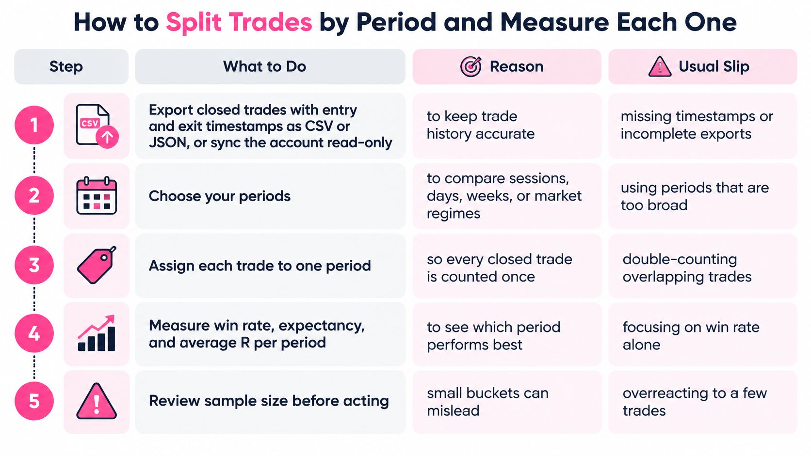
-
Export closed trades. Pull entry and exit timestamps as CSV or JSON, or sync the account read-only, then export again after the sync finishes. Trade history syncs every 15 minutes, and balance and position data syncs every 60 minutes, so an export taken in the middle of a sync can miss the latest fills. The usual slip is a file with prices and no timestamps.
-
Convert every timestamp to UTC. Mixing exchange local time with your laptop clock is the most common reason session results look random. One missed offset moves a London open into the Asia bucket.
-
Tag each trade once. Mark session, weekday, weekend flag, and week of month. A trade that spans two sessions belongs to the session where it opened. Double-counting the overlap is how one winner inflates two rows.
-
Count closed trades per bucket and mark any bucket under its minimum. Leave thin buckets in the sheet, but do not promote them.
-
Calculate the full metric row for each bucket that clears the floor: trade count, win rate, average R-multiple, expectancy, profit factor, maximum drawdown, and average holding time. Focusing on win rate alone is the slip that makes a small-winner bucket look like a schedule change.
-
Put the overall baseline in the first row of one results table. Every later row should be readable against that baseline, not against the best bucket you found.
-
Flag only clear gaps. Carry forward buckets that differ from the baseline by a margin you would trade, and that still hold enough closed trades. Park the rest.
The short walkthrough below shows the same export-and-tag flow on a live log if you want to see the columns before you build them.
Keep the raw export. If a later tag rule changes, you rebuild the buckets from the file instead of editing numbers in the summary.
Take a log of 120 closed trades over six months. London shows 38 trades, a 55% win rate, and expectancy of +0.31R. Asia shows 29 trades, a 34% win rate, and expectancy of −0.12R. Friday shows 14 trades and a 64% win rate. The chart makes London look like the strategy and Friday look like a gift.
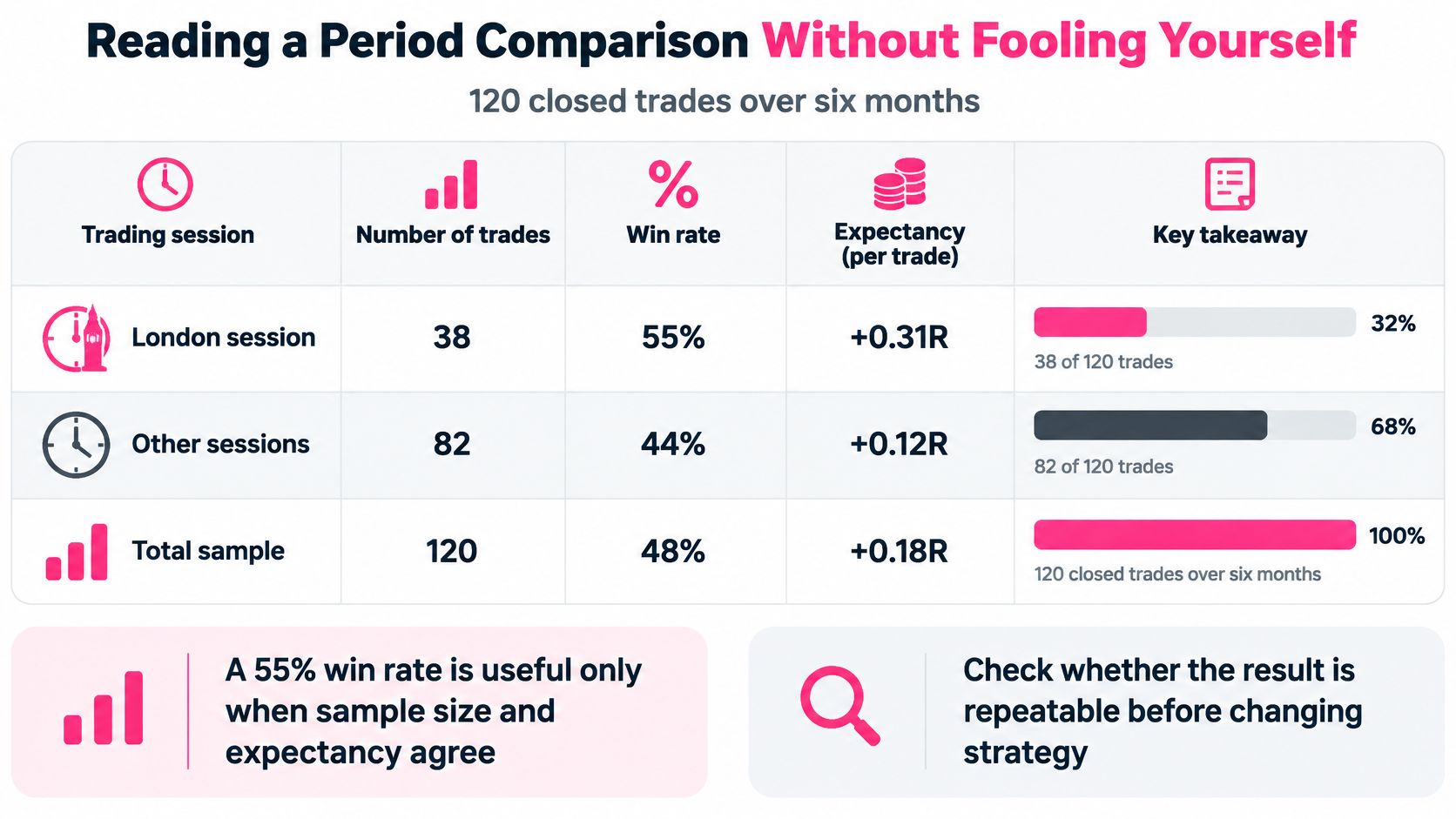
A 55% win rate is useful only when sample size and expectancy agree. Three checks decide whether you keep, watch, or test.
Split the period in half. London stays positive in both halves, so the gap is not one hot month. Asia is negative in the first half and flat in the second, so it passes this check only in the weak sense that it never turns into a clear winner.
Remove the three largest winners. London's expectancy stays positive, so one lucky fill is not carrying the bucket. Asia stays negative. Friday's win rate collapses once those winners leave, which tells you the percentage was a couple of trades.
Tag market condition by hand. Mark trending weeks and ranging weeks, then see whether the gap holds in both. London does. Asia does not separate cleanly. Friday has too few trades in either tag to say anything.
Friday fails the sample test. Fourteen trades is a hypothesis to watch, not a rule to trade. London passes all three checks and earns a forward test. Asia goes on the watch list because it failed the outlier and regime checks. You have not proved that London hours cause the edge. You have shown the gap is repeatable enough to test with new trades.
Check whether the result is repeatable before changing strategy. A bar that looks decisive on 14 trades is still a small sample wearing a large percentage.
A clean bucket can still lie. A spectrogram shows when energy moved; the cause still has to be supplied by the analyst. The same caution applies to a trade log: quantile time-frequency connectedness research finds that return relationships in extreme-return quantiles can differ materially from relationships near the median, so one global correlation plot can hide regime asymmetry. Even strong benchmark results in related research do not, by themselves, prove causal or tradable edge.
The same log can look profitable in one window and unprofitable in another because each split changes the sample as much as the clock. Narrow the window and a few fills dominate the average. Widen it and a good regime gets diluted by a bad one. The trap is treating that sampling choice as a discovery about time itself.
Multiple comparisons. If you slice by hour, weekday, session, and regime until one bar looks strong, chance will eventually sponsor a winner. Name the slices before opening the results, and treat every slice you did not name as a hypothesis for later testing.
Mixed strategies. Results shift after you changed the rule halfway through the period because two systems are sitting in one bucket. The hour is only where the rule change happened to land. Start a new period whenever the strategy changes, and tag the reason for the change while the trade is still fresh.
Correlation mistaken for cause. A London edge can vanish once setup type is controlled, which means the hour may reflect the setups you chose to trade then. Compare the same setup across periods before blaming the clock. Overlapping windows can also leak the same trade into two slices and invent a link that was never in the market.
Look-ahead bias. A rule looks strong when the test reuses the data that shaped it. Choose buckets and rules on the first half of the log, then test them on the second half. A test that reuses its design data flatters the rule. Thin samples create a related trap, which is why sample size in crypto trading belongs in the same review as the split itself.
| Pitfall |
Symptom |
Why it misleads |
Fix |
| Multiple comparisons |
One of many buckets looks strong |
Checking many slices makes one look good by chance |
Fix the buckets before reviewing results |
| Mixed strategies |
Results shift after a rule change mid-period |
Two systems are merged into one bucket |
Start a new period when the strategy changes |
| Correlation mistaken for cause |
A London edge that vanishes once setup type is controlled |
The hour may reflect the setups traded |
Compare the same setup across periods |
| Look-ahead bias |
A rule that looks strong only on the data used to design it |
The test reuses the data that shaped the rule |
Choose rules on the first half and test on the second |
A time bucket is a lens. Change the focal length and the same log tells a different story, so the job is to prove the story survives a new sample before the schedule changes.
Change one variable. Pick a single bucket that passed every check and already holds at least 20 closed trades. Write a rule that is specific enough to fail. Two versions that qualify: cut position size during the Asia session for the next 20 closed trades in that session, or skip new Friday entries until that weekday reaches 20 closed trades and you have rerun the checks.
Write the rule down before the first trade under it. If you edit the wording after a bad week, you are no longer testing the idea you chose. Tag every trade made under the rule, keep the log in CSV or JSON, and compare the test window with the prior window using the same metric row: count, win rate, average R, expectancy, profit factor, drawdown, and holding time.
Review by trades, not by calendar days. A quiet fortnight can deliver four fills and a loud week can deliver twenty. Set the trigger at a fixed count, such as 20 new closed trades in that bucket, then decide keep, drop, or run the same rule once more. Do not add a second change in the same test. If both size and session shift, you cannot tell which one moved expectancy.
Charts from 1 minute through 1 month, including 1m, 3m, 5m, 15m, 30m, 1H, 4H, 1D, 1W, and 1M, let you see whether the session you are testing even lines up with the timeframe you execute. A date-range measure between two points on the chart keeps the test window honest when you mark the start and the review. For the trade-count test itself, backtesting trading strategies is the right companion: design on one half, score on the other, and do not promote a bucket that only wins on the data that suggested it.
A period rule that survives 20 new trades is still a sample, not a law. It is large enough to keep, and small enough that you can drop it without rewriting the whole week.
Thrive is a trading journal that ties your closed trades to the market around them, so a session split sits next to the conditions you traded. Use the timing and performance views to test one period rule on your own log before you change when you show up. Start at Thrive and run the next 20 trades in that bucket against the baseline you wrote down today.